An Introduction to Contextual Bandits

In this post I discuss the Multi Armed Bandit problem and its applications to feed personalization. First, I will use a simple synthetic example to visualize arm selection in with bandit algorithms, I also evaluate the performance of some of the best known algorithms on a dataset for musical genre recommendations.
What is a Multi-Armed Bandit?
Imagine you have a bag full of biased coins. How would you go about finding the one that gives you the highest reward in expectation? You could use your favorite statistical tool by running enough independent trials to get a good estimate of the expected reward for each coin. This, of course, wouldn’t be realistic if you only had access to a limited amount of trials or if you had to pay a penalty every time you toss a coin and you get a bad outcome. If bias exploration is costly, you would need to be smarter about how you carry your experiments by somehow learning on the go and making sure that you explore all possibilities.
The biased coin scenario essentially captures the Multi-Armed Bandit (MAB) problem: A repeated game where the player chooses amongst a set of available arms, and at every point of the game he/she can only see the outcome of the action that was chosen. Although highly restrictive, the assumption that only rewards for chosen actions can be observed is much closer to many real-life situations:
- Clinical trial where there is no way to know what the results would have been if a patient had received a different treatment
- Sponsored ad placement on a website since it is always difficult to estimate what the clickthrough-rate would have been if we had chosen a different ad
- Choosing to eat chicken noodle soup instead of tomato soup
The MAB has been successfully used to make personalized news recommendation, test image placement on websites and optimizing random allocation in clinical trials. In most machine learning applications, bandit algorithms are used for making smart choices on highly dynamical settings where the pool of available options is rapidly changing and the set of actions to choose has a limited lifespan.
Arm Exploration vs Arm Exploitation
I used John Myle’s implementation of Bandit Algorithms to illustrate how we can tackle the biased coin problem using a MAB. For illustration purposes, we will use Normally distributed rewards instead of Bernoulli trials. I am assuming that we can choose between eight arms, where each arm draws from a normal distribution with the following parameters.
| Arms | Arm 1 | Arm 2 | Arm 3 | Arm 4 | Arm 5 | Arm 6 | Arm 7 | Arm 8 |
|---|---|---|---|---|---|---|---|---|
| Mean | 0.1 | 0.2 | 0.3 | 0.4 | 0.5 | 0.6 | 0.7 | 0.8 |
| Variance | 2 | 2 | 2 | 2 | 2 | 2 | 2 | 2 |
In this case, Arm 8 gives the highest reward; we want to test whether the algorithms correctly identify it. We will test the performance of two of the most well known MAB algorithms: ε-greedy and UCB1.
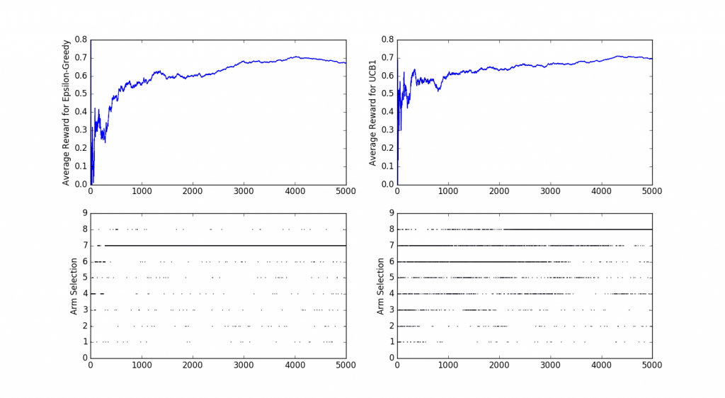
The image above shows the how the average reward and arm selection progresses over time for two MAB algorithms: ε-greedy and UCB1. There is an initial period of exploration and after a while, the algorithms converge to their preferred strategy. In this case, ε-Greedy quickly converges to the second-best solution (Arm 7) and UCB1 slowly converges to the optimal strategy. Note how both algorithms tend to concentrate on a small subset of available arms but they never stop exploring all possible options. By keeping the exploration step alive we make sure that we are still choosing the best action but in the process, we fail to exploit the optimal strategy to its fullest, this captures the Exploration-vs-Exploitation dilemma that is often found in bandit problems.
Why is exploration useful even when we have identified an optimal arm? In the next experiment, I replicated the same scenario as before, but I have included a distributional shift at t=2500 where the optimal choice becomes Arm 1. The shift in distributions is summarized in the following table:
|Arms| Arm 1|Arm 2 |Arm 3| Arm 4|Arm 5 |Arm 6|Arm 7 |Arm 8|
| –|–|–|–| –|–|–|–|–|–|
| Mean|8 |6 |7 |4 |3 |2|1 |5|
| Variance|2|2|2|2|2|2|2|2|
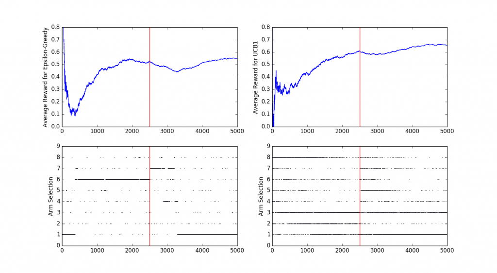
The graph shows how both ε-greedy and UCB1 adapt to a change in reward distribution. For this specific simulation, UCB1 quickly adapted to the new optimal arm, whereas ε-greedy was a bit slower to adapt (note how the Average Reward curve dips a little bit after the change in distribution takes place). As always, we should take these results with a grain of salt and not try to draw too many conclusions from one simulation, if you are interested in experimenting with different parameters feel free to tweak the script that I used to generate these results.
Contextual Bandits
In most real-life applications, we have access to information that can be used to make a better decision when choosing amongst all actions in a MAB setting, this extra information is what gives Contextual Bandits their name. For the ad-placement example, having access to historical data about the user’s buying habits can be highly informative of what type of products or promotions they will engage with in the future. There are many algorithms that deal with contextual Bandits , let’s start with the most popular one :
- Linear UCB :
The UCB algorithm is a very attractive algorithm for finite-action stochastic bandits: It is near-minimax optimal and is also almost instance optimal for any finite horizon and even asymptotically. It is thus quite natural to attempt to generalize UCB to the linear settings.
The generalization is based on the view that UCB implements the optimism in the face of uncertainty principle, according to which one should choose the actions as if the environment (in our case the linear bandit environment) was as nice as plausible possible. In finite-action stochastic bandit problems the principle dictates to choose the action with the largest upper confidence bound. In the case of linear bandit problems this still holds, but now to calculate the upper confidence bounds one should also better take into account the information conveyed by all the rewards observed because all the data (A1,X1,…,At−1,Xt−1)(A1,X1,…,At−1,Xt−1) is now connected through the unknown parameter vector. I highly recommend to check this article for more information about the mathematical aspect . You can find my implementation of the algorithm in this link .
- Epsilon - greedy :
Exploit the best strategy with probability 1-epsilon, keep exploring uniformly over all the other actions with probability epsilon.
- Contextual Thompson Sampling
Thompson Sampling works by maintaining a prior on the the mean rewards of its arms. In this, it follows a beta-binomial model with parameters alpha and beta, sampling values for each arm from its prior and picking the arm with the highest value. When an arm is pulled and a Bernoulli reward is observed, it modifies the prior based on the reward. This procedure is repeated for the next arm pull. You can find my implementation of the algorithm in this link