Reinforcement Q-learning

---

Most of you have probably heard of AI learning to play computer games on their own, a very popular example being Deepmind. Deepmind hit the news when their AlphaGo program defeated the South Korean Go world champion in 2016. There had been many successful attempts in the past to develop agents with the intent of playing Atari games like Breakout, Pong, and Space Invaders.

Each of these programs follow a paradigm of Machine Learning known as Reinforcement Learning. If you’ve never been exposed to reinforcement learning before, the following is a very straightforward analogy for how it works.

1- Reinforcement Learning Analogy

Consider the scenario of teaching a dog new tricks. The dog doesn’t understand our language, so we can’t tell him what to do. Instead, we follow a different strategy. We emulate a situation (or a cue), and the dog tries to respond in many different ways. If the dog’s response is the desired one, we reward them with snacks. Now guess what, the next time the dog is exposed to the same situation, the dog executes a similar action with even more enthusiasm in expectation of more food. That’s like learning “what to do” from positive experiences. Similarly, dogs will tend to learn what not to do when face with negative experiences.

That’s exactly how Reinforcement Learning works in a broader sense:

• Your dog is an “agent” that is exposed to the environment. The environment could in your house, with you.
• The situations they encounter are analogous to a state. An example of a state could be your dog standing and you use a specific word in a certain tone in your living room
• Our agents react by performing an action to transition from one “state” to another “state,” your dog goes from standing to sitting, for example.
• After the transition, they may receive a reward or penalty in return. You give them a treat! Or a “No” as a penalty.
• The policy is the strategy of choosing an action given a state in expectation of better outcomes.

Reinforcement Learning lies between the spectrum of Supervised Learning and Unsupervised Learning, and there’s a few important things to note:

1. Being greedy doesn’t always work
   There are things that are easy to do for instant gratification, and there’s things that provide long term rewards The goal is to not be greedy by looking for the quick immediate rewards, but instead to optimize for maximum rewards over the whole training.

2. Sequence matters in Reinforcement Learning
   The reward agent does not just depend on the current state, but the entire history of states. Unlike supervised and unsupervised learning, time is important here.

2-The Reinforcement Learning Process

In a way, Reinforcement Learning is the science of making optimal decisions using experiences. Breaking it down, the process of Reinforcement Learning involves these simple steps:

1. Observation of the environment
2. Deciding how to act using some strategy
3. Acting accordingly
4. Receiving a reward or penalty
5. Learning from the experiences and refining our strategy
6. Iterate until an optimal strategy is found

Let’s now understand Reinforcement Learning by actually developing an agent to learn to play a game automatically on its own.

3- Enter Reinforcement Learning

We are going to use a simple RL algorithm called Q-learning which will give our agent some memory.

Intro to Q-learning

Essentially, Q-learning lets the agent use the environment’s rewards to learn, over time, the best action to take in a given state.

In our Taxi environment, we have the reward table, P, that the agent will learn from. It does thing by looking receiving a reward for taking an action in the current state, then updating a Q-value to remember if that action was beneficial.

The values store in the Q-table are called a Q-values, and they map to a (state, action) combination.

A Q-value for a particular state-action combination is representative of the “quality” of an action taken from that state. Better Q-values imply better chances of getting greater rewards.

For example, if the taxi is faced with a state that includes a passenger at its current location, it is highly likely that the Q-value for pickup is higher when compared to other actions, like dropoff or north.

Q-values are initialized to an arbitrary value, and as the agent exposes itself to the environment and receives different rewards by executing different actions, the Q-values are updated using the equation:

Q(state,action)←(1−α)Q(state,action)+α(reward+γmaxaQ(next state,all actions))Q(state,action)←(1−α)Q(state,action)+α(reward+γmaxaQ(next state,all actions))

Where:

• αα (alpha) is the learning rate (0<α≤10<α≤1) - Just like in supervised learning settings, αα is the extent to which our Q-values are being updated in every iteration.

• γγ (gamma) is the discount factor (0≤γ≤10≤γ≤1) - determines how much importance we want to give to future rewards. A high value for the discount factor (close to 1) captures the long-term effective award, whereas, a discount factor of 0 makes our agent consider only immediate reward, hence making it greedy.

What is this saying?

We are assigning (←←), or updating, the Q-value of the agent’s current state and action by first taking a weight (1−α1−α) of the old Q-value, then adding the learned value. The learned value is a combination of the reward for taking the current action in the current state, and the discounted maximum reward from the next state we will be in once we take the current action.

Basically, we are learning the proper action to take in the current state by looking at the reward for the current state/action combo, and the max rewards for the next state. This will eventually cause our taxi to consider the route with the best rewards strung together.

The Q-value of a state-action pair is the sum of the instant reward and the discounted future reward (of the resulting state). The way we store the Q-values for each state and action is through a Q-table

Q-Table

The Q-table is a matrix where we have a row for every state (500) and a column for every action (6). It’s first initialized to 0, and then values are updated after training. Note that the Q-table has the same dimensions as the reward table, but it has a completely different purpose.

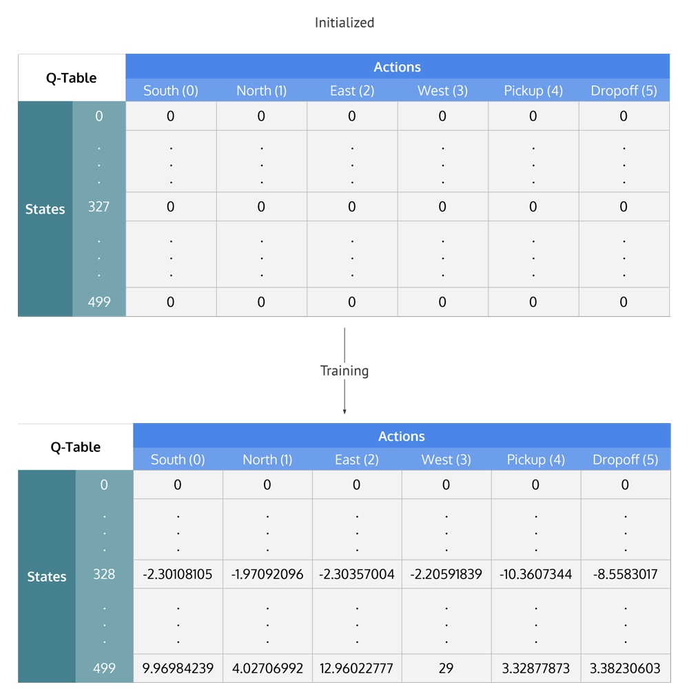
Q-Table values are initialized to zero and then updated during training to values that optimize the agent’s traversal through the environment for maximum rewards

Summing up the Q-Learning Process

Breaking it down into steps, we get

• Initialize the Q-table by all zeros.
• Start exploring actions: For each state, select any one among all possible actions for the current state (S).
• Travel to the next state (S’) as a result of that action (a).
• For all possible actions from the state (S’) select the one with the highest Q-value.
• Update Q-table values using the equation.
• Set the next state as the current state.
• If goal state is reached, then end and repeat the process.

Exploiting learned values

After enough random exploration of actions, the Q-values tend to converge serving our agent as an action-value function which it can exploit to pick the most optimal action from a given state.

There’s a tradeoff between exploration (choosing a random action) and exploitation (choosing actions based on already learned Q-values). We want to prevent the action from always taking the same route, and possibly overfitting, so we’ll be introducing another parameter called ϵϵ “epsilon” to cater to this during training.

Instead of just selecting the best learned Q-value action, we’ll sometimes favor exploring the action space further. Lower epsilon value results in episodes with more penalties (on average) which is obvious because we are exploring and making random decisions.

Implementing Q-learning in python

Training the Agent

First, we’ll initialize the Q-table to a 500×6500×6 matrix of zeros:

import numpy as np
q_table = np.zeros([env.observation_space.n, env.action_space.n])  

We can now create the training algorithm that will update this Q-table as the agent explores the environment over thousands of episodes.

In the first part of while not done, we decide whether to pick a random action or to exploit the already computed Q-values. This is done simply by using the epsilon value and comparing it to the random.uniform(0, 1) function, which returns an arbitrary number between 0 and 1.

We execute the chosen action in the environment to obtain the next_state and the reward from performing the action. After that, we calculate the maximum Q-value for the actions corresponding to the next_state, and with that, we can easily update our Q-value to the new_q_value:

%%time """Training the agent"""  
import random from  IPython.display 
import clear_output # Hyperparameters 
import gym

# import env
env = gym.make("Taxi-v2").env
env.render()


alpha =  0.1 
gamma =  0.6 
epsilon =  0.1 
 # For plotting metrics 
all_epochs =  [] 
all_penalties =  [] 
for i in range(1,  100001): 
	state = env.reset() 
	epochs, penalties, reward,  =  0,  0,  0 
	done =  False  
	while  not done:  
		if random.uniform(0,  1)  < epsilon:
			 action = env.action_space.sample()  # Explore action space  
		else: 
			action = np.argmax(q_table[state])  # Exploit learned values 	 
		next_state, reward, done, info = env.step(action) 
		old_value = q_table[state, action] 
		next_max = np.max(q_table[next_state]) 
		new_value =  (1  - alpha)  * old_value + alpha *  (reward + gamma * next_max) 
		q_table[state, action]  = new_value 
		if reward ==  -10: 
			penalties +=  1 
		state = next_state
	    epochs +=  1  
	  if i %  100  ==  0: 
		  clear_output(wait=True)  
		  print(f"Episode: {i}")  
	  print("Training finished.\n")  

OUT:

Episode:  100000  Training finished.  Wall time:  30.6 s 

Now that the Q-table has been established over 100,000 episodes, let’s see what the Q-values are at our illustration’s state:

q_table[328]  

OUT:

array([  -2.30108105,  -1.97092096,  -2.30357004,  -2.20591839,  -10.3607344  ,  -8.5583017  ])  

The max Q-value is “north” (-1.971), so it looks like Q-learning has effectively learned the best action to take in our illustration’s state!