1- An explanation of the Bayesian approach to linear modeling
The Bayesian vs Frequentist debate is one of those academic arguments that I find more interesting to watch than engage in. Rather than enthusiastically jump in on one side, I think it’s more productive to learn both methods of statistical inference and apply them where appropriate. In that line of thinking, recently, I have been working to learn and apply Bayesian inference methods to supplement the frequentist statistics covered in my grad classes.
One of my first areas of focus in applied Bayesian Inference was Bayesian Linear modeling. The most important part of the learning process might just be explaining an idea to others, and this post is my attempt to introduce the concept of Bayesian Linear Regression. We’ll do a brief review of the frequentist approach to linear regression, introduce the Bayesian interpretation, and look at some results applied to a simple dataset. The full code can be found on GitHub in a Jupyter Notebook.
2- Recap of Frequentist Linear Regression
The frequentist view of linear regression is probably the one you are familiar with from school: the model assumes that the response variable (y) is a linear combination of weights multiplied by a set of predictor variables (x). The full formula also includes an error term to account for random sampling noise. For example, if we have two predictors, the equation is:
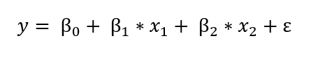
y is the response variable (also called the dependent variable), β’s are the weights (known as the model parameters), x’s are the values of the predictor variables, and ε is an error term representing random sampling noise or the effect of variables not included in the model.
Linear Regression is a simple model which makes it easily interpretable: β_0 is the intercept term and the other weights, β’s, show the effect on the response of increasing a predictor variable. For example, if β_1 is 1.2, then for every unit increase in x_1,the response will increase by 1.2.
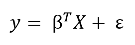
We can generalize the linear model to any number of predictors using matrix equations. Adding a constant term of 1 to the predictor matrix to account for the intercept, we can write the matrix formula as:
The goal of learning a linear model from training data is to find the coefficients, β, that best explain the data. In frequentist linear regression, the best explanation is taken to mean the coefficients, β, that minimize the residual sum of squares (RSS). RSS is the total of the squared differences between the known values (y) and the predicted model outputs (ŷ, pronounced y-hat indicating an estimate). The residual sum of squares is a function of the model parameters:
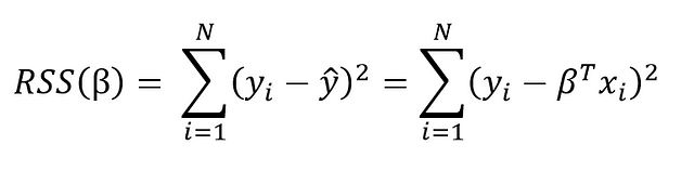
The summation is taken over the N data points in the training set. We won’t go into the details here (check out this reference for the derivation), but this equation has a closed form solution for the model parameters, β, that minimize the error. This is known as the maximum likelihood estimate of β because it is the value that is the most probable given the inputs, X, and outputs, y. The closed form solution expressed in matrix form is:
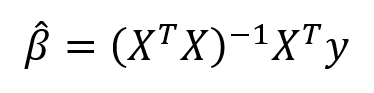
(Again, we have to put the ‘hat’ on β because it represents an estimate for the model parameters.) Don’t let the matrix math scare you off! Thanks to libraries like Scikit-learn in Python, we generally don’t have to calculate this by hand (although it is good practice to code a linear regression). This method of fitting the model parameters by minimizing the RSS is called Ordinary Least Squares (OLS).
What we obtain from frequentist linear regression is a single estimate for the model parameters based only on the training data. Our model is completely informed by the data: in this view, everything that we need to know for our model is encoded in the training data we have available.
Once we have β-hat, we can estimate the output value of any new data point by applying our model equation:

As an example of OLS, we can perform a linear regression on real-world data which has duration and calories burned for 15000 exercise observations. Below is the data and OLS model obtained by solving the above matrix equation for the model parameters:

With OLS, we get a single estimate of the model parameters, in this case, the intercept and slope of the line.We can write the equation produced by OLS:
calories = -21.83 + 7.17 * duration
From the slope, we can say that every additional minute of exercise results in 7.17 additional calories burned. The intercept in this case is not as helpful, because it tells us that if we exercise for 0 minutes, we will burn -21.86 calories! This is just an artifact of the OLS fitting procedure, which finds the line that minimizes the error on the training data regardless of whether it physically makes sense.
If we have a new datapoint, say an exercise duration of 15.5 minutes, we can plug it into the equation to get a point estimate of calories burned:
calories = -21.83 + 7.17 * 15.5 = 89.2
Ordinary least squares gives us a single point estimate for the output, which we can interpret as the most likely estimate given the data. However, if we have a small dataset we might like to express our estimate as a distribution of possible values. This is where Bayesian Linear Regression comes in.
3- Bayesian Linear Regression
In the Bayesian viewpoint, we formulate linear regression using probability distributions rather than point estimates. The response, y, is not estimated as a single value, but is assumed to be drawn from a probability distribution. The model for Bayesian Linear Regression with the response sampled from a normal distribution is:
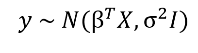
The output, y is generated from a normal (Gaussian) Distribution characterized by a mean and variance. The mean for linear regression is the transpose of the weight matrix multiplied by the predictor matrix. The variance is the square of the standard deviation σ (multiplied by the Identity matrix because this is a multi-dimensional formulation of the model).
The aim of Bayesian Linear Regression is not to find the single “best” value of the model parameters, but rather to determine the posterior distribution for the model parameters. Not only is the response generated from a probability distribution, but the model parameters are assumed to come from a distribution as well. The posterior probability of the model parameters is conditional upon the training inputs and outputs:
![]()
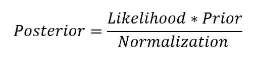
| Here, P(β | y, X) is the posterior probability distribution of the model parameters given the inputs and outputs. This is equal to the likelihood of the data, P(y | β, X), multiplied by the prior probability of the parameters and divided by a normalization constant. This is a simple expression of Bayes Theorem, the fundamental underpinning of Bayesian Inference: |
Let’s stop and think about what this means. In contrast to OLS, we have a posterior distribution for the model parameters that is proportional to the likelihood of the data multiplied by the prior probability of the parameters. Here we can observe the two primary benefits of Bayesian Linear Regression.
- Priors: If we have domain knowledge, or a guess for what the model parameters should be, we can include them in our model, unlike in the frequentist approach which assumes everything there is to know about the parameters comes from the data. If we don’t have any estimates ahead of time, we can use non-informative priors for the parameters such as a normal distribution.
- Posterior: The result of performing Bayesian Linear Regression is a distribution of possible model parameters based on the data and the prior. This allows us to quantify our uncertainty about the model: if we have fewer data points, the posterior distribution will be more spread out.
As the amount of data points increases, the likelihood washes out the prior, and in the case of infinite data, the outputs for the parameters converge to the values obtained from OLS.
The formulation of model parameters as distributions encapsulates the Bayesian worldview: we start out with an initial estimate, our prior, and as we gather more evidence, our model becomes less wrong. Bayesian reasoning is a natural extension of our intuition. Often, we have an initial hypothesis, and as we collect data that either supports or disproves our ideas, we change our model of the world (ideally this is how we would reason)!
4- Computing posteriors in Python
4.1 Recall of the context
To begin with, let’s assume we have a one-dimensional dataset (x1,y1),…,(xk,yk)(x1,y1),…,(xk,yk). The goal is to predict yi as a function of xi. Our model describing yi is
where α and β are unknown parameters, and e is the statistical noise. In the Bayesian approach, α and β are unknown, and all we can do is form an opinion (compute a posterior) about what they might be.
To start off, we’ll assume that our observations are independent and identically distributed. This means that for every ii, we have that: where each ei is a random variable. Let’s assume that ei is an absolutely continuous random variable, which means that it has a probability density function given by E(t).
Our goal will be to compute a posterior on (α,β), i.e. a probability distribution p(α,β) that represents our degree of belief that any particular (α,β) is the “correct” one.
At this point it’s useful to compare and contrast standard linear regression to the bayesian variety.
In standard linear regression, your goal is to find a single estimator α
In bayesian linear regression, you get a probability distribution representing your degree of belief as to how likely α is. Then for any unknown x, you get a probability distribution on y representing how likely y is. Specifically: Thinking probabilistically gave us several advantages; we can obtain the best values of α and β (the same as with optimization methods) together with the uncertainty estimation of those parameters. Optimization methods require extra work to provide this information. Additionally, we get the flexibility of Bayesian methods, meaning we will be able to adapt our models to our particular problems; for example, moving away from normality assumptions, or building hierarchical linear models
4.2 PyMC3 introduction
PyMC3 is a Python library for probabilistic programming. The last version at the moment of writing is 3.0.rc2 released on October 4th, 2016. PyMC3 provides a very simple and intuitive syntax that is easy to read and that is close to the syntax used in the statistical literature to describe probabilistic models. PyMC3 is written using Python, where the computationally demanding parts are written using NumPy and Theano. Theano is a Python library originally developed for deep learning that allows us to define, optimize, and evaluate mathematical expressions involving multidimensional arrays efficiently. The main reason PyMC3 uses Theano is because some of the sampling methods, like NUTS, need gradients to be computed and Theano knows how to do automatic differentiation. Also, Theano compiles Python code to C code, and hence PyMC3 is really fast. This is all the information about Theano we need to have to use PyMC3. If you still want to learn more about it start reading the official Theano tutorial at http://deeplearning.net/software/ theano/tutorial/index.html#tutorial.
4.3 Uniform Prior
To compute the posteriors on (α,β) in Python, we first import the PyMC library:
import pymc3 as pm
import numpy as np
import pandas as pd
from theano import shared
import scipy.stats as stats
import matplotlib.pyplot as plt
import arviz as az
az.style.use('arviz-darkgrid')
We then generate our data set (since this is a simulation), or otherwise load it from an original data source:
from scipy.stats import norm

k = 100 #number of data points
x_data = norm(0,1).rvs(k)
y_data = x_data + norm(0,0.35).rvs(k) + 0.5
We then define priors on (α,β)(α,β). In this case, we’ll choose uniform priors on [-5,5]:
alpha = pm.Uniform('alpha', lower=-5, upper=5)
beta = pm.Uniform('beta', lower=-5, upper=5)
Finally, we define our observations.
x = pm.Normal('x', mu=0,tau=1,value=x_data, observed=True)
@pm.deterministic(plot=False)
def linear_regress(x=x, alpha=alpha, beta=beta):
    return x*alpha+beta

y = pm.Normal('output', mu=linear_regress, value=y_data, observed=True)
Note that for the values x and y, we’ve told PyMC that these values are known quantities that we obtained from observation. Then we run to some Markov Chain Monte Carlo:
model = pm.Model([x, y, alpha, beta])
mcmc = pm.MCMC(model)
mcmc.sample(iter=100000, burn=10000, thin=10)
We can then draw samples from the posteriors on alpha and beta:
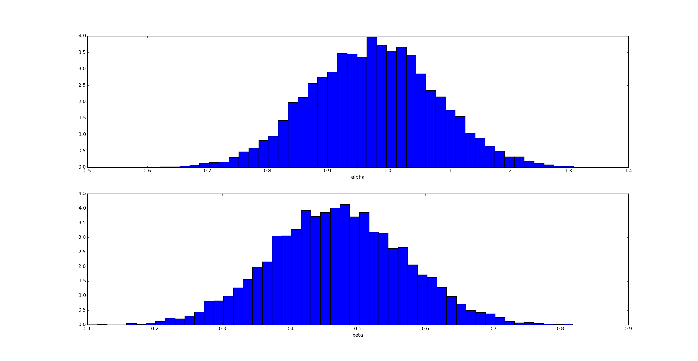
Unsurprisingly (given how we generated the data) the posterior for αα is clustered near α=1 and for β near β=0.5.
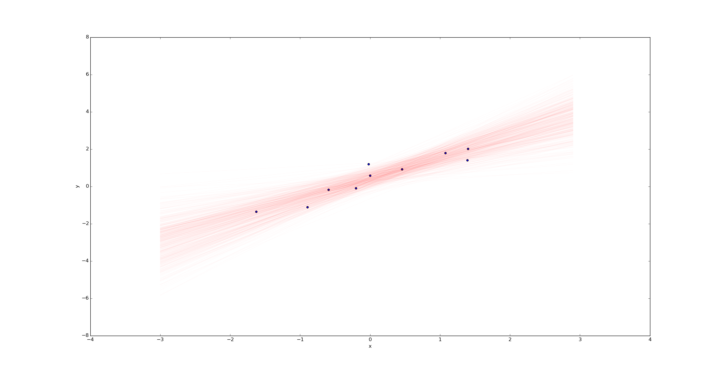
We can then draw a sample of regression lines:
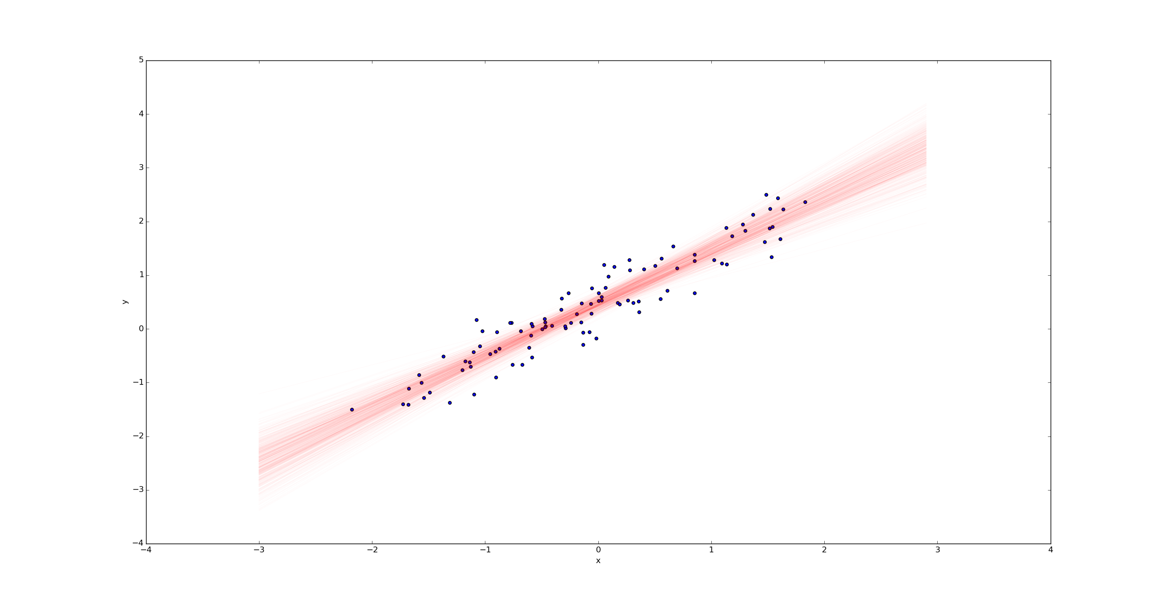
Unlike in the ordinary linear regression case, we don’t get a single regression line - we get a probability distribution on the space of all such lines. The width of this posterior represents the uncertainty in our estimate.
Imagine we were to change the variable k to k=10 in the beginning of the python script above. Then we would have only 10 samples (rather than 100) and we’d expect much more uncertainty. Plotting a sample of regression lines reveals this uncertainty:
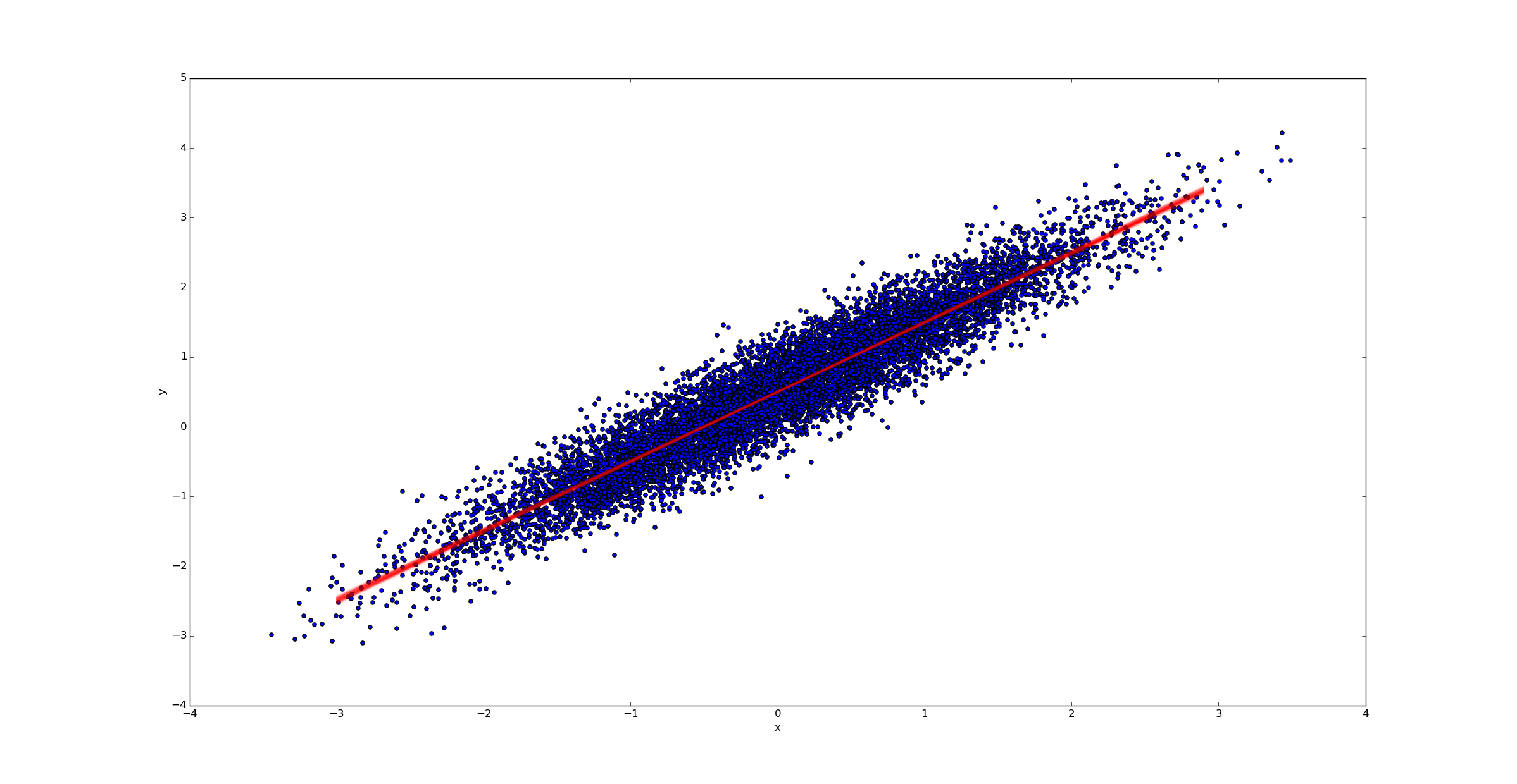
In contrast, if we had far more samples (say k=10000), we would have far less uncertainty in the best fit line:
4.5 Normal prior
Now we will change the prior. Once again we are going to rely on a synthetic data set to build intuition on the model. We will create the datasets in such a way that we know the values of the parameters that later we are going to try to find out.
np.random.seed(1)
N = 100
alpha_real = 2.5
beta_real = 0.9
eps_real = np.random.normal(0, 0.5, size=N)
x = np.random.normal(10, 1, N)
y_real = alpha_real + beta_real * x
y = y_real + eps_real
# we can center the data
#x = x - x.mean()
# or standardize the data
#x = (x - x.mean())/x.std()
#y = (y - y.mean())/y.std()
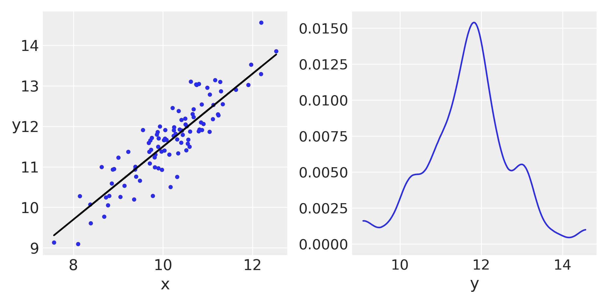
## plot
_, ax = plt.subplots(1, 2, figsize=(8, 4))
ax[0].plot(x, y, 'C0.')
ax[0].set_xlabel('x')
ax[0].set_ylabel('y', rotation=0)
ax[0].plot(x, y_real, 'k')
az.plot_kde(y, ax=ax[1])
ax[1].set_xlabel('y')
plt.tight_layout()
Now we use PyMC3 to fit the model, nothing we have not seen before :
with pm.Model() as model_g:
    α = pm.Normal('α', mu=0, sd=10)
    β = pm.Normal('β', mu=0, sd=1)
    ϵ = pm.HalfCauchy('ϵ', 5)

    μ = pm.Deterministic('μ', α + β * x)
	y_pred = pm.Normal('y_pred', mu=  α + β * x, sd=ϵ, observed=y
    trace_g = pm.sample(2000, tune=1000)
az.plot_trace(trace_g, var_names=['α', 'β', 'ϵ'])
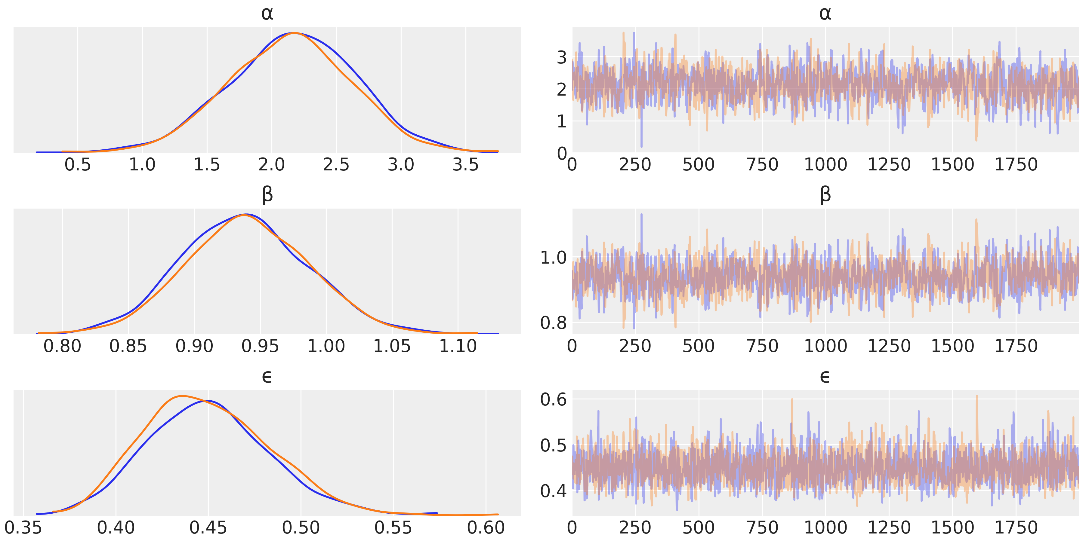
the KDE graphs are signaling good mixing !
Interpreting and visualizing the posterior
As we have already seen, we can explore the posterior using the PyMC3 functions, traceplot and df_summary, or we can use our own functions. For a linear regression it could be useful to plot the average line that fits the data together with the average mean values of α and β . We can also make a plot reflecting the posterior uncertainty using semitransparent lines sampled from the posterior:
plt.plot(x, y, 'C0.')

alpha_m = trace_g['α'].mean()
beta_m = trace_g['β'].mean()

draws = range(0, len(trace_g['α']), 10)
plt.plot(x, trace_g['α'][draws] + trace_g['β'][draws]
         * x[:, np.newaxis], c='gray', alpha=0.5)

plt.plot(x, alpha_m + beta_m * x, c='k',
         label=f'y = {alpha_m:.2f} + {beta_m:.2f} * x')

plt.xlabel('x')
plt.ylabel('y', rotation=0)
plt.legend()
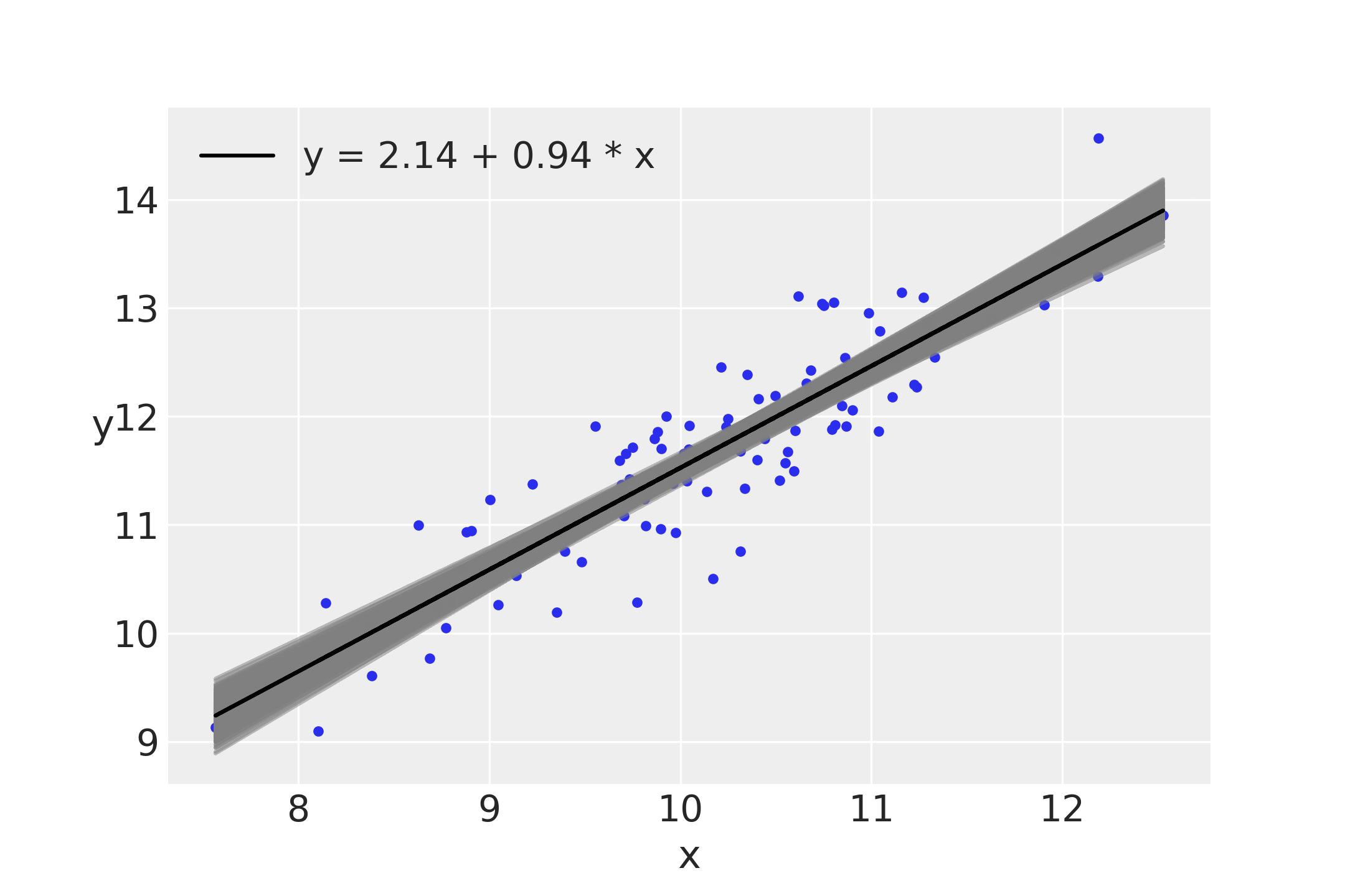
Notice that uncertainty is lower in the middle, although it is not reduced to a single point; that is, the posterior is compatible with lines not passing exactly for the mean of the data, as we have already mentioned