Hypothesis Testing
Statistics is all about coming up with models to explain what is going on in the world. But how good are we at that? I mean, numbers are only good for so many things, right? How do we know if they are telling the right story?
Today I will give a brief introduction over this topic which created headache for me when I started to learn machine learning and econometrics . I will try to clarify the different concepts about hypothesis testing and illustrate their use throughout some examples in python , So let’s enter the famous world of test statistics !!
1 Statistical and Hypothesis Testing
The goal of a test statistic is to determine how well the model fits the data and whether there is a significant difference between groups. Think of it a little like clothing. When you are in the store, the mannequin tells you how the clothes are supposed to look (the theoretical model). When you get home, you test them out and see how they actually look (the data-based model). The test-statistic tells you if the difference between them (because I definitely do not look like the mannequin.) is significant. Generally , we use the term Hypothesis testing because we basically made an assumption about the model or the population parameters and then we look for some mathematical conclusion what ever we are assuming is true or not .
Example : you say the avg student in class is 20 or the unployment is correlated to inflation by 1.92 . To do so , we need a measure or a kind of confidence interval that tell us how far these hypothesis are true .
2 The basic of hypothesis testing ?
2.1 Normal Distribution
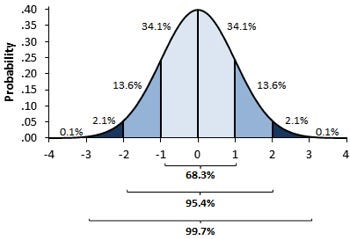
A variable is said to be normally distributed or have a normal distribution if its distribution has the shape of a normal curve — a special bell-shaped curve. … The graph of a normal distribution is called the normal curve
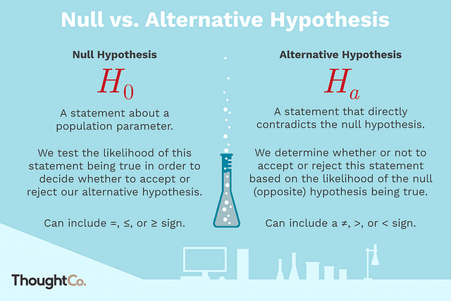
2.2 Null and Alternative hypothesis :
In inferential statistics, the null hypothesis is a general statement or default position that there is no relationship between two measured phenomena, or no association among groups In other words it is a basic assumption or made based on domain or problem knowledge.
Example : a company production is = 50 unit/per day etc.
The alternative hypothesis is the hypothesis used in hypothesis testing that is contrary to the null hypothesis. It is usually taken to be that the observations are the result of a real effect (with some amount of chance variation superposed)
Example : a company production is !=50 unit/per day etc.
2.3 Level of significance:
Refers to the degree of significance in which we accept or reject the null-hypothesis. 100% accuracy is not possible for accepting or rejecting a hypothesis, so we therefore select a level of significance that is usually 5%.
This is normally denoted with alpha(maths symbol ) and generally it is 0.05 or 5% , which means your output should be 95% confident to give similar kind of result in each sample.
2.4 One tailed test : A test of a statistical hypothesis , where the region of rejection is on only one side of the sampling distribution , is called a one-tailed test.
Example :- a college has ≥ 4000 student or data science ≤ 80% org adopted.
2.5 Two-tailed test :- A two-tailed test is a statistical test in which the critical area of a distribution is two-sided and tests whether a sample is greater than or less than a certain range of values. If the sample being tested falls into either of the critical areas, the alternative hypothesis is accepted instead of the null hypothesis.
Example : a college != 4000 student or data science != 80% org adopted
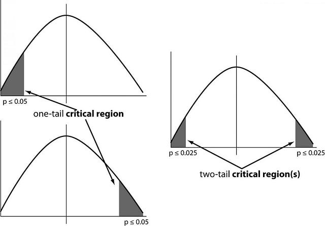
one and two-tailed images
2.6 P-value :
The P value, or calculated probability, is the probability of finding the observed, or more extreme, results when the null hypothesis (H 0) of a study question is true — the definition of ‘extreme’ depends on how the hypothesis is being tested.
If your P value is less than the chosen significance level then you reject the null hypothesis i.e. accept that your sample gives reasonable evidence to support the alternative hypothesis. It does NOT imply a “meaningful” or “important” difference; that is for you to decide when considering the real-world relevance of your result.
Example : you have a coin and you don’t know whether that is fair or tricky so let’s decide null and alternate hypothesis
H0 : a coin is a fair coin.
H1 : a coin is a tricky coin. and alpha = 5% or 0.05
Now let’s toss the coin and calculate p- value ( probability value).
Toss a coin 1st time and result is tail- P-value = 50% (as head and tail have equal probability)
Toss a coin 2nd time and result is tail, now p-value = 50/2 = 25%
and similarly we Toss 6 consecutive time and got result as P-value = 1.5% but we set our significance level as 95% means 5% error rate we allow and here we see we are beyond that level i.e. our null- hypothesis does not hold good so we need to reject and propose that this coin is a tricky coin which is actually.
Now Let’s see some of widely used hypothesis testing type :
- T Test ( Student T test)
- Z Test
- ANOVA Test
- Chi-Square Test
- Chow test
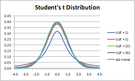
3- T-test
A t-test is a type of inferential statistic which is used to determine if there is a significant difference between the means of two groups which may be related in certain features. It is mostly used when the data sets, like the set of data recorded as outcome from flipping a coin a 100 times, would follow a normal distribution and may have unknown variances. . The t test also tells you how significant the differences are; In other words it lets you know if those differences could have happened by chance.
3.1 What is t-score?
The t score is a ratio between the difference between two groups and the difference within the groups. The larger the t score, the more difference there is between groups. The smaller the t score, the more similarity there is between groups. A t score of 3 means that the groups are three times as different from each other as they are within each other. When you run a t test, the bigger the t-value, the more likely it is that the results are repeatable.
- A large t-score tells you that the groups are different.
- A small t-score tells you that the groups are similar.
3.2 What are T-Values and P-values?
How big is “big enough”? Every t-value has a p-value to go with it. A p-value is the probability that the results from your sample data occurred by chance. P-values are from 0% to 100%. They are usually written as a decimal. For example, a p value of 5% is 0.05. Low p-values are good; They indicate your data did not occur by chance. For example, a p-value of .01 means there is only a 1% probability that the results from an experiment happened by chance. In most cases, a p-value of 0.05 (5%) is accepted to mean the data is valid.
3.3 Types of t-tests?
There are **three main types of t-test:
- An Independent Samples t-test compares the means for two groups.
- A Paired sample t-test compares means from the same group at different times (say, one year apart).
- A One sample t-test tests the mean of a single group against a known mean.
3.3 How to perform a 2 sample t-test?
Lets us say we have to test whether the height of men in the population is different from height of women in general. So we take a sample from the population and use the t-test to see if the result is significant.
Steps:
- Determine a null and alternate hypothesis
In general, the null hypothesis will state that the two populations being tested have no statistically significant difference. The alternate hypothesis will state that there is one present. In this example we can say that:

- Collect sample data
Next step is to collect data for each population group. In our example we will collect 2 sets of data, one with the height of women and one with the height of men. The sample size should ideally be the same but it can be different. Lets say that the sample sizes are nx and ny.
- Determine a confidence interval and degrees of freedom
This is what we call alpha (α). The typical value of α is 0.05. This means that there is 95% confidence that the conclusion of this test will be valid. The degree of freedom can be calculated by the the following formula:

- Calculate the t-statistic
t-statistic can be calculated using the below formula:
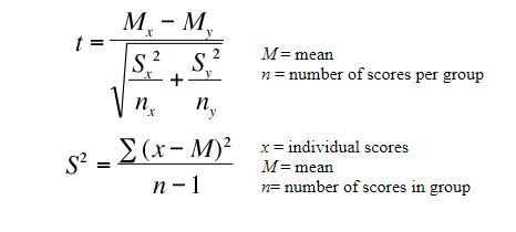
where, Mx and My are the mean values of the two samples of male and female.
Nx and Ny are the sample space of the two samples
S is the standard deviation
- Calculate the critical t-value from the t distribution
To calculate the critical t-value, we need 2 things, the chosen value of alpha and the degrees of freedom. The formula of critical t-value is complex but it is fixed for a fixed pair of degree of freedom and value of alpha. We therefore use a table to calculate the critical t-value:
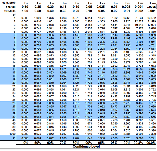
In python, rather than looking up in the table we will use a function from the sciPy package. (I promise u, its the only time we will use it!)
- Compare the critical t-values with the calculated t statistic
If the calculated t-statistic is greater than the critical t-value, the test concludes that there is a statistically significant difference between the two populations. Therefore, you reject the null hypothesis that there is no statistically significant difference between the two populations.
In any other case, there is no statistically significant difference between the two populations. The test fails to reject the null hypothesis and we accept the alternate hypothesis which says that the height of men and women are statistically different.
## Import the packages
import numpy as np
from scipy import stats


## Define 2 random distributions
#Sample Size
N = 10
#Gaussian distributed data with mean = 2 and var = 1
a = np.random.randn(N) + 2
#Gaussian distributed data with with mean = 0 and var = 1
b = np.random.randn(N)


## Calculate the Standard Deviation
#Calculate the variance to get the standard deviation

#For unbiased max likelihood estimate we have to divide the var by N-1, and therefore the parameter ddof = 1
var_a = a.var(ddof=1)
var_b = b.var(ddof=1)

#std deviation
s = np.sqrt((var_a + var_b)/2)
s


## Calculate the t-statistics
t = (a.mean() - b.mean())/(s*np.sqrt(2/N))


## Compare with the critical t-value
#Degrees of freedom
df = 2*N - 2

#p-value after comparison with the t
p = 1 - stats.t.cdf(t,df=df)


print("t = " + str(t))
print("p = " + str(2*p))
### You can see that after comparing the t statistic with the critical t value (computed internally) we get a good p value of 0.0005 and thus we reject the null hypothesis and thus it proves that the mean of the two distributions are different and statistically significant.


## Cross Checking with the internal scipy function
t2, p2 = stats.ttest_ind(a,b)
print("t = " + str(t2))
print("p = " + str(p2))


```


# 4- Anova Test
we introduced the t-test for checking whether the means of two groups differ.The t-test works when dealing with two groups, but sometimes we want to compare more than two groups at the same time. For example, if we wanted to test whether voter age differs based on some categorical variable like race, we have to compare the means of each level or group the variable. We could carry out a separate t-test for each pair of groups, but when you conduct many tests you increase the chances of false positives. The [analysis of variance](https://en.wikipedia.org/wiki/Analysis_of_variance) or ANOVA is a statistical inference test that lets you compare multiple groups at the same time.


The one-way ANOVA tests whether the mean of some numeric variable differs across the levels of one categorical variable. It essentially answers the question: do any of the group means differ from one another? We won't get into the details of carrying out an ANOVA by hand as it involves more calculations than the t-test, but the process is similar: you go through several calculations to arrive at a test statistic and then you compare the test statistic to a critical value based on a probability distribution. In the case of the ANOVA, you use the "[f-distribution](https://en.wikipedia.org/wiki/F-distribution)".

The scipy library has a function for carrying out one-way ANOVA tests called scipy.stats.f_oneway(). Let's generate some fake voter age and demographic data and use the ANOVA to compare average ages across the groups:

````python
import numpy as np
import pandas as pd
import matplotlib.pyplot as plt
import scipy.stats as stats
np.random.seed(12)

races =   ["asian","black","hispanic","other","white"]

# Generate random data
voter_race = np.random.choice(a= races,
                              p = [0.05, 0.15 ,0.25, 0.05, 0.5],
                              size=1000)

voter_age = stats.poisson.rvs(loc=18,
                              mu=30,
                              size=1000)

# Group age data by race
voter_frame = pd.DataFrame({"race":voter_race,"age":voter_age})
groups = voter_frame.groupby("race").groups

# Etract individual groups
asian = voter_age[groups["asian"]]
black = voter_age[groups["black"]]
hispanic = voter_age[groups["hispanic"]]
other = voter_age[groups["other"]]
white = voter_age[groups["white"]]

# Perform the ANOVA
stats.f_oneway(asian, black, hispanic, other, white)
F_onewayResult(statistic=1.7744689357289216, pvalue=0.13173183202014213)
The test output yields an F-statistic of 1.774 and a p-value of 0.1317, indicating that there is no significant difference between the means of each group.
5. Chi-Squared Test
In our study of t-tests, we introduced the one-way t-test to check whether a sample mean differs from the an expected (population) mean. The chi-squared goodness-of-fit test is an analog of the one-way t-test for categorical variables: it tests whether the distribution of sample categorical data matches an expected distribution. For example, you could use a chi-squared goodness-of-fit test to check whether the race demographics of members at your church or school match that of the entire U.S. population or whether the computer browser preferences of your friends match those of Internet uses as a whole.
When working with categorical data, the values themselves aren’t of much use for statistical testing because categories like “male”, “female,” and “other” have no mathematical meaning. Tests dealing with categorical variables are based on variable counts instead of the actual value of the variables themselves.
Let’s generate some fake demographic data for U.S. and Minnesota and walk through the chi-square goodness of fit test to check whether they are different:
import numpy as np
import pandas as pd
import scipy.stats as stats
national = pd.DataFrame(["white"]*100000 + ["hispanic"]*60000 +\
                        ["black"]*50000 + ["asian"]*15000 + ["other"]*35000)


minnesota = pd.DataFrame(["white"]*600 + ["hispanic"]*300 + \
                         ["black"]*250 +["asian"]*75 + ["other"]*150)

national_table = pd.crosstab(index=national[0], columns="count")
minnesota_table = pd.crosstab(index=minnesota[0], columns="count")

print( "National")
print(national_table)
print(" ")
print( "Minnesota")
print(minnesota_table)
Chi-squared tests are based on the so-called chi-squared statistic. You calculate the chi-squared statistic with the following formula:
sum((observed−expected) ²/ expected)
In the formula, observed is the actual observed count for each category and expected is the expected count based on the distribution of the population for the corresponding category. Let’s calculate the chi-squared statistic for our data to illustrate:
observed = minnesota_table

national_ratios = national_table/len(national)  # Get population ratios

expected = national_ratios * len(minnesota)   # Get expected counts

chi_squared_stat = (((observed-expected)**2)/expected).sum()

print(chi_squared_stat)
col_0 count 18.194805 dtype: float64
*Note: The chi-squared test assumes none of the expected counts are less than 5.
Similar to the t-test where we compared the t-test statistic to a critical value based on the t-distribution to determine whether the result is significant, in the chi-square test we compare the chi-square test statistic to a critical value based on the chi-square distribution. The scipy library shorthand for the chi-square distribution is chi2. Let’s use this knowledge to find the critical value for 95% confidence level and check the p-value of our result:
crit = stats.chi2.ppf(q = 0.95, # Find the critical value for 95% confidence*
                      df = 4)   # Df = number of variable categories - 1

print("Critical value")
print(crit)

p_value = 1 - stats.chi2.cdf(x=chi_squared_stat,  # Find the p-value
                             df=4)
print("P value")
print(p_value)
Critical value 9.48772903678 P value [ 0.00113047]
*Note: we are only interested in the right tail of the chi-square distribution. Read more on this here.
Since our chi-squared statistic exceeds the critical value, we’d reject the null hypothesis that the two distributions are the same.
6- Chow test
A Chow test is designed to determine whether a structural break in a time series exists. That is to say, a sharp change in trend in a time series that merits further study. For instance, a structural break in one series can give useful clues as to whether such a change is being propagated across other variables – assuming that there is a significant correlation between them under normal circumstances.
 The Chow test is conducted by running three separate regressions: 1) a pooled regression with data before and after the structural break, 2) a regression with data before the structural break, and 3) a regression with data after the structural break. The residual sum of squares for each regression is used to calculate the Chow statistic using the following formula:
CHOW = (RSSP - (RSSA+RSSB))/k) / (RSSA+RSSB)/(NA+NB-2k) where RSS = Residual Sum of Squares k = number of regressors (including intercept) N = degrees of freedom
Note that this test can be set up automatically in R using the “strucchange” package. However, I always prefer to calculate the test statistic manually where possible, as it facilitates understanding of why we are applying the test, along with understanding the specific break that we are analysing in the time series.
The null and alternative hypothesis is as follows:
-
Null Hypothesis: No structural break in time series
-
Alternative Hypothesis: Structural break in time series
At the outset, let me say that the Chow Test is more of an academic model in nature, and is not as commonly used as other time series methods. Firstly, most time series (especially ones with an economic or financial trend involved) will show many structural breaks. The Chow Test is mainly useful when it comes to analysing structural breaks across time series that are normally stationary, but a significant shift causes a break in the series.